Binary Search
Engineering is about trade-offs. Different tools make sense for different problems. There are
very few things with no utility under any circumstance. I want to belabour
this point in this post using a very simple example - binary search.
Binary search is an efficient way to find an element (called the key) in an array of elements. The caveat is - the array must be sorted. The cost of doing binary search on a sorted array is $O(log N)$ where N is the size of the array. Most things in this world are sorted only because someone put an effort into it - think the dictionary of words. Therefore, binary search demands that we pay the cost of sorting upfront. The cost of sorting is $O(N. log N)$.
We will contrast it with linear search. Linear search suggests we scan the array until we find the element. In worst case, the cost of linear search is $O(N)$ per look up.
We want to find out for what size of array and for how many planned look-ups does binary search makes sense and under which one must stick to linear search.
Let's set up our equation.
For what values of K and N does binary search make sense ?§
We want to find the point beyond which the cost of doing linear search exceeds the cost of binary search with a one time cost of sorting. Say, we assume the size of the array is $N$ and the number of look-ups is $k$.
$$ Nlog(N) + k.log(N) \le kN $$
$$ or, Nlog(N) \le k(N - log(N)) $$
$$ or, k \ge \frac{Nlog(N)}{N-log(N)} $$
$$ or, k \ge \frac{log (N)}{1- \frac{log(N)}{N}} $$
The math says that if the number of lookups is greater than $\frac{log (N)}{1- \frac{log(N)}{N}}$, then we should consider binary search and under which a linear scan should be preferred.
Now let's plot this.
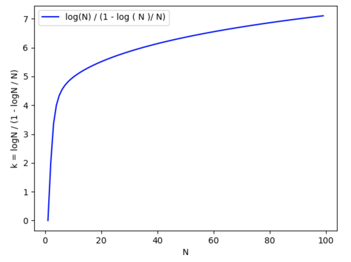
Along the x axis we have different sizes of arrays. On the Y-axis we have the number of lookups beyond which binary search makes sense. For example, if we have an array of size 100 and we are going to look-up at least seven times, we should consider sorting the array and doing a binary-search.
But say, you have an array of size 20 and you are going to do just 2 lookups, you are better off scanning it both the times.
Appendix§
Binary Search implementation.§
def binary_search(key: int, arr: list[int]) -> int:
    """
    Find the index of the key in the sorted list if it exists,
    or return -1.
    """

    lo, hi = 0, len(arr) - 1

    # The equality is important or else you will miss the key, if it were the last element of the sorted array.
    while lo <= hi:
        # Find the index of the middle element.
        mid = lo + (hi - lo) // 2

        if arr[mid] == key:
            return mid
        elif arr[mid] < key:
            # too small
            lo = mid + 1
        else:
            # mid is too high
            hi = mid - 1
    return -1
Python code for the plot§
import math
from matplotlib import pyplot as plt

X_MAX = 1000
Y = 1

# The denominator.
one_minus_logn_over_n = [(x, 1 - math.log2(x) / x) for x in range(1, X_MAX)]

# The term on the right side of in-equality.
log_n_over_one_minus_logn_over_n = [
    (x, math.log2(x) / (1 - math.log2(x) / x)) for x in range(1, X_MAX)
]

# Ploting log x, just to show that it becomes the dominating function for large values of x
logn = [(x, math.log2(x)) for x in range(1, X_MAX)]

# This is to show what the denominator converges to for large values of X
xys2 = [(x, Y) for x in range(1, X_MAX)]

plt.scatter(
    *zip(*one_minus_logn_over_n), color="red", label="1 - log ( N )/ N"
)

plt.plot(
    *zip(*log_n_over_one_minus_logn_over_n),
    "-",
    color="blue",
    label="log(N) / (1 - log ( N )/ N)",
)
plt.scatter(*zip(*logn), color="orange", label="log ( N )")
plt.plot(*zip(*xys2), "-.", color="green", label=f"y = {Y}")

plt.xlabel("X")
plt.ylabel("f(N)")
plt.legend()